An overview of how LLMs work (chp1):

Large Language Models (LLMs) work in three big steps:

Training on massive text

• They’re fed huge amounts of text (books, code, websites).
• The model learns patterns: grammar, facts, reasoning shortcuts, styles of writing.
• The core task is predicting the next word in a sequence.

Neural network architecture (Transformers)

• Built on the Transformer model.
• Uses self-attention to decide which words in a sentence matter most to each other.
• Multiple layers of attention and feedforward networks build complex representations of text.

Inference (using the model)

• Given a prompt, the model encodes it into vectors.
• It predicts the most likely next token (word/part of word) repeatedly.

Chapter 2

2.1 understanding word embeddings

Embeddings are just convertin non numerical data (such as text) into numeric data - this is called word embedding. map each word to a numeric data. Also there's sentence or paragraph embeddings - mapping sentences/paras to numeric data (used in RAG btw)

word2vec is an embedding model that would figure out the word embeddings by predicting the context of that word given the target or by predicting the target given the context (exact details idk man)
words that appear in similar contexts tend to have similar meaning
Pretrained models are used to generate embeddings for ML models, llms however have their own embeddings in the input layer and are updated during training. Well why not just use word2vec?? here's the thing if you train your own embedding model then you have your data fitting into your context - it will match more with the context of you training data instead of something generic that word2vec will likely produce

Even the smallest gpt2 models with 117M and 125M parameters use an embedding size of 768 dimensions. GPT3 with 175b parameters uses 12,288 dimensions (sheesh)

Summary:

• Embeddings is the process of converting words/sentences(depends) into vectors
• word2vec is a pretrained neural network normally used to generate embeddings for ml models
• llms usually do not use word2vec. They have their own embeddings in the input layer. Think of llms as one neural network - everything is happening within

2.2 tokenizing text

now forget embeddings for a while, you need to tokenize text first.

• each word is a token, each special character is a token
• each whitespace is skipped, all others are split into tokens\

so you:

• downloaded the verdict, read it
• to understand tokenization, you write a regex that will split words on each whitespace (to get singular words)
• some words are connected with a punctuation so you're now splitting each punctuation mark too.
• now loop through each and remove whitespace tokens for the simplicity

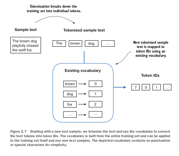
2.3 converting tokens into token ids

In this step you will convert all tokens into token ids. This step comes before converting the token ids into embedding vectors. So far;

• split text into tokens
• convert into token ids
• then comes 'embeddings'
  To convert into token ids;
• just grab all words, create a set to remove duplicates
• use enumerate to assign a number to each and create a dict object - call it vocab
• now we'll use this vocab to convert all the tokens into token ids. You have a map, now you transform everything according to that map.

At this point, you have a list of token_ids adjacent to each token so you can convert your original list of tokens into token_ids. Now well you need the opposite as well so you create a tokenizer class with an encode method that splits text into tokens and carries out the string-to-integer mapping to produce token IDs via the vocabulary and a decode method that carries out the reverse integer-to-string mapping to convert the token ids back into text. you create the SimpleTokenizerV1 class for this:

class SimpleTokenizerV1:
    def __init__(self, vocab):
        self.str_to_int = vocab
        self.int_to_str = { i:s for s,i in vocab.items() }

    def encode(self,text):
        preprocessed = re.split(r'([,.?_!"()\']|--|\s)', text)
        preprocessed = [item.strip() for item in preprocessed if item.strip()]
        ids = [self.str_to_int[s] for s in preprocessed]
        return ids

    def decode(self, ids):
        text = " ".join([self.int_to_str[i] for i in ids])
        text = re.sub(r'\s+([,.?!"()\'])', r'\1', text)
        return text
    

Now try using a word which is not available in the vocab - (book used 'hello') and you'll get an error because the vocab does not know what you're saying - as that word wasn't in the-verdict.txt

2.4 Special context tokens

In 2.3, you encountered an error because the token which was to be encoded wasn't available in vocab so now enters SimpleTokenizerV2 which will encode the words that aren't in vocab with a special token <| unk |>.

Also whenever concatenating text from different sources, use the <| end of text |> special token so that the model knows that these texts are separate - this will help in better 'next-word' prediction thingy as you will be separating the context.
Now, you take your existing vocab and add two more tokens in it, <| unk |> and <| end of text |>. then create tokenizerv2 as following:

class SimpleTokenizerV2:
    def __init__(self, vocab):
        self.str_to_int = vocab
        self.int_to_str = {i:s for s,i in vocab.items()}
    
    def encode(self, text):
        preprocessed = re.split(r'([,.:;?_!"()\']|--|\s)', text)
        preprocessed = [item.strip() for item in preprocessed if item.strip()]

        preprocessed = [item if item in self.str_to_int else "<|unk|>" for item in preprocessed]
        ids = [self.str_to_int[s] for s in preprocessed]
        return ids
    
    def decode(self, ids):
        text = " ".join([self.int_to_str[i] for i in ids])
        text = re.sub(r'\s+([,.:;?!"()\'])', r'\1', text)
        return text

tldr;

• For words out of vocab, use the <| unk |> token, and <| EOS |> or <| end of text|> for end of a sentence (helps model understand context)
• gpt tokenizer only uses <| end of text |> token for simplicity
• gpt tokenizer also doesn't use <| unk |> token for out of vocab words instead they use byte pair encoding which breaks down words into subwords

2.5 Byte Pair Encoding

(book doesn't go deep in this but i will, lol)

BPE looks at data then decides how to tokenize them, went ahead and found out the whole algorithm, it's relatively easy

for k times:
    - choose the most frequentyly adjacent symbols (suppose t and h are appearing together a lot)
    - replace every adjacent t and h with th - like link them together

note that bpe does not need the <| unk |> token as it is iteratively figuring out words and assigning tokens unlike the tokenizing approaches of SimpleTokenizerV2. If it encounters an unfamiliar word during tokenization, it can represent it as a sequence of subword tokens or characters. The ability to break down unknown words into individual characters ensures that the tokenizer and, consequently, the LLM that is trained with it can process any text, even if it contains words that were not present in its training data
(Normally used with tiktoken - library for tokenizing, duh?)

Just to recap, so far:

• split text into tokens
• use those tokens to create vocab i.e assign each token a token id
• convert all tokens into token ids
• created SimpleTokenizerV1 (without special tokens), SimpleTokenizerV2 (with special tokens) and then finally used tiktoken to just use BPE algorithm as BPE is much better at working with new words. if any word is not in its vocab, it will represent it as a collection of tokens

2.6 Data Sampling wih a sliding window

LLms are pretrained by predicting the next word in a text;

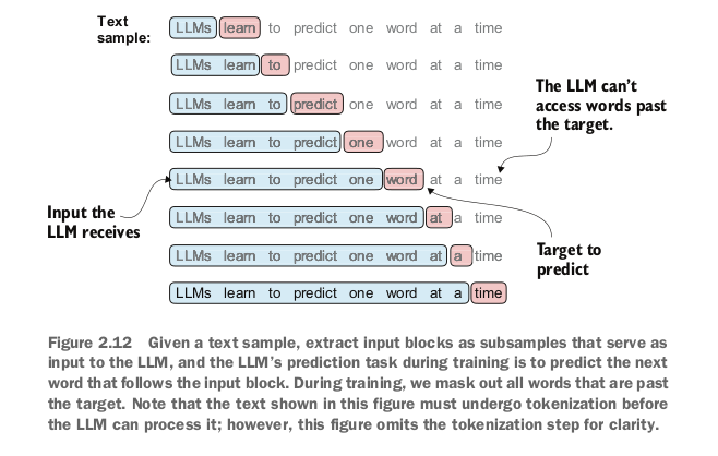
Next step is to create input-target pairs.
You accept a list of inputs then the model predicts the most likely next word for that list of inputs.

Input is the group of words you feed into an llm
target would be the word that it should predict

Sliding window Approach:

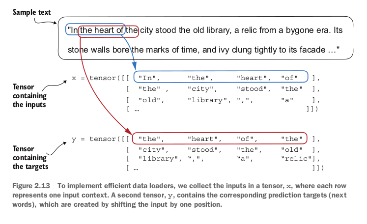
Read the-verdict.txt, and tokenize using bpe tokenizer The most intuitive ways to create the input-target pairs for the next word prediction task is to create two variables, x and y, where x contains the input tokens and y contains the targets, which are the inputs shifted by 1. Take a chunk of tokens, create x from 0:lastidx and then a y from 1:lastidx+1

context_size = 4
x = enc_sample[:context_size]
y = enc_sample[1:context_size+1]
print(f"x: {x}")
print(f"y:
{y}")

Here, context_size is how many tokens would be included in the input. context_size+ 1would be the target pairs

Data Loader and Dataset classes

One last step before turning tokens into embeddings: implementing an efficient data loader that iterates over the input dataset and returns the inputs and targets as PyTorch tensors, which can be thought of as multidimensional arrays

Creating this class to create input/target pairs in tensors with each tensor created by a skipping-token-amount of stride (if that makes sense):
Each row consists of a number of tokenIDs (based on max_length)

class GPTDatasetV1(Dataset):
    def __init__(self, txt, tokenizer, max_length, stride):
        self.input_ids = []
        self.target_ids = []

        token_ids = tokenizer.encode(txt)

        for i in range(0, len(token_ids) - max_length, stride):
            input_chunk = token_ids[i:1 + max_length]
            target_chunk = token_ids[i + 1: i + max_length + 1]
            self.input_ids.append(torch.tensor(input_chunk))
            self.target_ids.append(torch.tensor(target_chunk))

    
    def __len__(self):
        return len(self.input_ids)
    
    def __getitem__(self, idx):
        return self.input_ids[idx], self.target_ids[idx]

The code here was kinda complicating so just to recap:

• you're creating batches of input and target ids - call them chunks
• Think of each chunk as a tensor in figure 2.13. target chunk is 1 item shifted of input chunk
• stride is how many tokens you will skip through in the next iteration
• the other two methods are self-explanatory

After that, you just create a small function which works as an invoker/instantiator to the gptdatasetv1 class

def create_dataloader_v1(txt, batch_size=4, max_length=256, stride=128, shuffle=True, drop_last=True, num_workers=0):
    tokenizer = tiktoken.get_encoding("gpt2")
    dataset = GPTDatasetV1(txt, tokenizer, max_length, stride)

    dataloader = DataLoader(
        dataset,
        batch_size=batch_size,
        shuffle=shuffle,
        drop_last=drop_last,
        num_workers=num_workers
    )

    return dataloader

Now, if you need to use the GPTDatasetV1 class, you will do so with the create_dataloader_v1 method. GPTDatasetV1 will create the dataset and DataLoader will be also instantiated by the create_dataloader_v1 class.

Dataset Class : represents data - tells pytorch what the data is and how to access individual samples

DataLoader: provides a way to load batches of data with shuffling and parallel processing

max_length will tell you what the maximum number of items should be in each tensor(both input and output). Also note batch-size=1 results in tensor of length 1 (like 2d array, length1, inside the length1 you have max_length number of elements). Having a batch_size=8 will result in a tensor of length 8

Smaller batch sizes = Noisy model updates, which is why its normal to have batch sizes over atleast 256.
However,
Smaller batch sizes = less memory required during training, so batch size is a tradeoff to experiment wd

Also note, batch_size is the length of a tensor and max_length is the number of items in each inner list (coz multidimensioanl array, remember)

2.7 Create token embeddings

This is the last step. Embeddings are continuous vector representations and they're necessary since gpt-like llms are deep neural networks trained with the backpropagation algorithm. (idk how neural networks are trained with backpropagation algorithm and i dont have time right now so i'll use all my knowledge from reading that one AI history book and random geoffrey hinton articles i found on medium which is that you get to the output, then backtrace. Like go back, and adjusst the weights of that node which was activated to get to that output and if im not wrong you do this for each hidden layer)

To understand how token id to embedding vector conversion works, take four token ids, small vocab (6 words) and u want to create an embedding size of 3 (note that embedding size is dimensions and its normal to have a lott of those, gpt 3 has 12, 288 - jeez)

• embeddings are vector representation of tokens.

• In training, you have tokens, you assign a random embedding to all of them then you try predicting the next word in a sentence - this would mostly be wrong so you go back (back propagation) to figure where the error came from then you calculate loss and all to adjust embedding vector values plus some weights now your model is slightly better. repeat this a 1000 times until your model gets better.

• vocab_size and output_dim is the dimension of the resulting tensor embedding thingy

• embedding layer is the first real layer of the llm neural network except it's not a layer in the traditional sense - it works as a map. it has a tensor that contains one row per token id and that row is the adjacent embedding. It will map the token id resulting in an output of a 'continuous vector representation' or most commonly known as its gangsta name embedding

In other words, the embedding layer is essen- tially a lookup operation that retrieves rows from the embedding layer’s weight matrix via a token ID.

To recap, so far:

• you tokenize words
• you map them to a vocab providing a token id for each
• you have to now map them into input-target pairs
• then you use batches and stuff to come up with tensors with bunch of parameters such as max_length (max token per row), stride (how many tokens to skip before moving on to the next per batch) using Dataset class (responsible for creating effective datasets with proper batching and input/target pairs) and a DataLoader class which will aid in fetching input/target tensors one by one
• then finally, you convert these input tensors into embedding layeer. You already know the outputs (input/target pairs, remember?) so you're gonna help the llm learn better which inputs are to be mapped to which outputs. Note that embeddings are assumed at first then gradually adjusted during the training process

2.8 Encoding word positions

The token id remains the same regardless of it's position and regardless of how far apart it is. Now you can think of a problem here, imagine two sentences "I dont think this is working" and "I like this", the position of "this" and "i" in both of the sentences has variable lengths but the words in both of these sentences will have the same token id. "this" in sentence 1 and sentence 2 will have the same token id even though they are used in different contexts and you can see how the model will have probs figuring out what words to pay attention to if they just have the same token ids.

To solve this, there's two broad categories of position-aware embeddings (embeddings unlike the ones described above, they are aware of the "context" so to speak)

• Absolute Positional Embeddings:
  . Absolute Positional Embeddings are directly associated with specific positions in a sequence.

• Relative Positional Embeddings:
  Relative positional embeddings will tell you relationships based on how far apart instead of "at wihch exact position". this will help generalizing better to variable sequence length

(GPT models use absolute positional embeddings, instead of fixed positional encodings in the original transformer model)

To implement this, follow the following steps:

• Load raw text from "the-verdict.txt"
• Define vocabulary size and embedding dimension
• Create an embedding layer to map token IDs to 256-dimensional vectors
• Tokenize text and prepare batches using create_dataloader_v1, with sliding windows
• Fetch one batch of input and target token IDs
• Convert token IDs to embeddings via the token embedding layer
• Create a positional embedding layer for max_length positions
• Generate absolute positional embeddings (one per position index)
• Add token and positional embeddings together to get final input embeddings for

Chapter 2 Summary:

Summary

• LLMs require textual data to be converted into numerical vectors, known as embeddings, since they can’t process raw text. Embeddings transform discrete data (like words or images) into continuous vector spaces, making them com- patible with neural network operations.
• As the first step, raw text is broken into tokens, which can be words or characters. Then, the tokens are converted into integer representations, termed token IDs.
• Special tokens, such as <|unk|> and <|endoftext|>, can be added to enhance the model’s understanding and handle various contexts, such as unknown words or marking the boundary between unrelated texts. the model
• The byte pair encoding (BPE) tokenizer used for LLMs like GPT-2 and GPT-3 can efficiently handle unknown words by breaking them down into subword units or individual characters.
• We use a sliding window approach on tokenized data to generate input–target pairs for LLM training.
• Embedding layers in PyTorch function as a lookup operation, retrieving vectors corresponding to token IDs. The resulting embedding vectors provide continuous representations of tokens, which is crucial for training deep learning mod- els like LLMs.
• While token embeddings provide consistent vector representations for each token, they lack a sense of the token’s position in a sequence. To rectify this, two main types of positional embeddings exist: absolute and relative. OpenAI’s GPT models utilize absolute positional embeddings, which are added to the token embedding vectors and are optimized during the model training.

Chapter 3

So far, tokenize text, convert into token ids, create embeddings. Now comes the attention mechanism part 4 variants of attention mechanism covered:

1. Simplified self attention
2. Self attention
3. Causal attention
4. Multi-head attention

3.1 The problem with modeling long sequences:

consider translating two languages, there are often occurrences where a sentence cannot be mapped word by word to another language as each language has its own semantics and certain words go at certain positions which isnt necessarily uniform among all languages. you can imagine, a translating neural network not being efficient if all its doing is translating each word without context.

To solve this problem, neural networks with encoder and decoders are used. The encoder reads the entire text and processes it and then the decoder produces the translated text. Before transformers, RNNs were used where outouts from previous steps are fed as inputs to the current step

The big limitation of encoder–decoder RNNs is that the RNN can’t directly access earlier hidden states from the encoder during the decoding phase. Consequently, it relies solely on the current hidden state, which encapsulates all relevant information. This can lead to a loss of context, especially in complex sentences where dependen- cies might span long distances.

3.2 Capturing data dependencies with attention mechanisms

RNNs wont work well for longer texts - but will work fine for shorter sentences. The problem is that RNN would not have a wider context of previous words in the input. The rnn must remember the entire encoeded in out iin a single hidden state before passing it to the decoder

To solve this, came bahdanau attention mechanism that had attention mechanism built in into it, but later everyone realized 'hey, we dont nned rnns' and enter transformer architecture with a self attention mechanism

3.3 Attending to different parts of the input with self attention:

3.3.1

The idea here is to create context vectors such that each element of a sequence (consider the phrase "Your Journey Starts") where each word is represented by x(i) and we have to calculate z(i) for all x(i) which is sort of a map for one word and its relation to all others if that makes sense

To illustrate this concept, let’s focus on the embedding vector of the second input element, x(2) (which corresponds to the token “journey”), and the corresponding con- text vector, z(2), shown at the bottom of figure 3.7. This enhanced context vector, z(2), is an embedding that contains information about x(2) and all other input elements, x(1) to x(T).

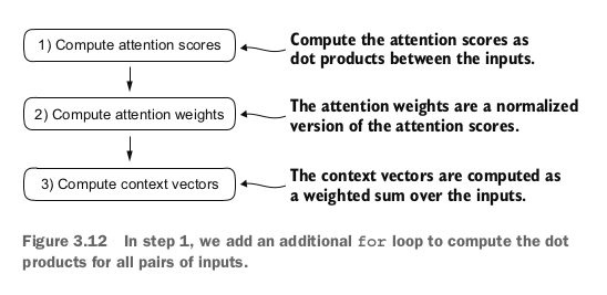
The first step of implementing self-attention is to compute intermediate values ω referred to as attention scores and for each input vector x(1), you compute relevant attention scores by finding out the dot product between the input vector x(1) and other input vector {x(2), x(3)}

In the next step, we normalize each of the attention scores we computed previously You have to obtain attention weights that must sum up to 1 - thus the normalization.

To normalize, divide each attention weight you calculated by the sum of all attention weights - doing so will result in a sum of all attention weights = 1

query = inputs[1]
attn_scores_2 = torch.empty(inputs.shape[0])
for i, x_i in enumerate(inputs):
    attn_scores_2[i] = torch.dot(x_i, query)
print(attn_scores_2)

attn_weights_2_tmp = attn_scores_2 / attn_scores_2.sum()
print("Attention weights:", attn_weights_2_tmp)
print("Sum:", attn_weights_2_tmp.sum())

Normalization can be done by using the softmax function, whose basic implementation is as follows:

def softmax_naive(x):
    return torch.exp(x) / torch.exp(x).sum(dim=0)

attn_weights_2_naive = softmax_naive(attn_scores_2)
print("Attention weights:", attn_weights_2_naive)
print("Sum:", attn_weights_2_naive.sum())

In addition, the softmax function ensures that the attention weights are always posi- tive. This makes the output interpretable as probabilities or relative importance, where higher weights indicate greater importance.

However the naive softmax algorithm may run into problems as overflow or underflow when dealing with large or small input values - which is why pytorch's softmax is much better

attn_weights_2 = torch.softmax(attn_scores_2, dim=0)
print("Attention weights:", attn_weights_2)
print("Sum:", attn_weights_2.sum())

Now since we have already calculated attention weights,we'll now calculate context vector - and you do that by multiplication of input tokens x(i) by their corresponding attention weights and then summing the resulting vectors. Thus, context vector z(2) is the weighted sum of all input vectors, obtained by multiplying each input vector by its corresponding attention weight:

query = inputs[1]
context_vec_2 = torch.zeros(query.shape)
for i,x_i in enumerate(inputs):
    context_vec_2 += attn_weights_2[i]*x_i
print(context_vec_2)

Next, we will generalize this procedure for computing context vectors to calculate all context vectors simultaneously.

3.3.2 Computing Attention weights for all input tokens

So far, we calculated attention weigths and context vector for input 2 so we're doing it for each input now Modified code to compute all context vectors:

attn_scores = torch.empty(6, 6)
for i, x_i in enumerate(inputs):
    for j, x_j in enumerate(inputs):
        attn_scores[i, j] = torch.dot(x_i, x_j)
print(attn_scores)

The resulting attention scores look a lil like this:

tensor([[0.9995, 0.9544, 0.9422, 0.4753, 0.4576, 0.6310],
[0.9544, 1.4950, 1.4754, 0.8434, 0.7070, 1.0865],
[0.9422, 1.4754, 1.4570, 0.8296, 0.7154, 1.0605],
[0.4753, 0.8434, 0.8296, 0.4937, 0.3474, 0.6565],
[0.4576, 0.7070, 0.7154, 0.3474, 0.6654, 0.2935],
[0.6310, 1.0865, 1.0605, 0.6565, 0.2935, 0.9450]])